Examples
Below, we present some examples to illustrate the usages of PyNOL.
A quick start
First, we give a simple example that employs Online Gradient Descent (OGD) algorithm to optimize the fixed online loss functions \(f_t(x) = {\sum}_{i=1}^d x_i^2, \forall t \in [T]\), where \(d\) is the dimension and \(T\) is the number of rounds.
import matplotlib.pyplot as plt
import numpy as np
from pynol.environment.environment import Environment
from pynol.environment.domain import Ball
from pynol.learner.base import OGD

T, dimension, step_size, seed = 100, 10, 0.01, 0
domain = Ball(dimension=dimension, radius=1.)  # define the unit ball as the feasible set
ogd = OGD(domain=domain, step_size=step_size, seed=seed)
env = Environment(func=lambda x: (x**2).sum())
loss = np.zeros(T)
for t in range(T):
    _, loss[t], _ = ogd.opt(env)
plt.plot(loss)
plt.savefig('quick_start.pdf')
Then, we can visualize the instantaneous loss of the online learning process as follows.

Use predefined algorithms
Then, we embark on a tour of PyNOL exemplifying online linear regression with square loss. The data \((\varphi_t, y_t)_{t=1,\cdots,T}\) are generated by model parameters \(x_t^* \in \mathcal{X}\) with label \(y_t = \varphi_t^\top {x}_t^* + \epsilon_t\), where feature \(\varphi_t\) and model parameter \(x_t^*`\) are sampled randomly and uniformly in the \(d\)-dimension unit ball, \(\epsilon_t \sim \mathcal{N}(\mu, \sigma)\) is the Gaussian noise. To simulate the non-stationary environments, we generate a piecewise-stationary process with \(S`\) stages, where \(x_t^*\) is fixed at each stage and changes randomly among different stages. At iteration \(t\), the learner receives feature \(\varphi_t\), then predicts \(\hat{y}_t = \varphi_t^\top x_t\) according to the current model \(x_t \in \mathcal{X}\). We choose square loss \(\ell(y, \hat{y})=\frac{a}{2}(y-\hat{y})^2\), so online function \(f_t: \mathcal{X} \mapsto \mathbb{R}`\) is the composition of loss function and data item, i.e., \(f_t(x) = \ell(y_t, \hat{y}_t)=\frac{\alpha}{2}(y_t-\varphi_t^\top x)^2\). We set \(T=10000\), \(d=3\), \(S=100\), \(\mu=0\), \(\sigma = 0.05\) and set \(\alpha=1/2\) to ensure the loss is bounded by \([0, 1]\).
Generate data for experiments. We provide synthetic data generator in
utils/data_generator, which includingLinearRegressionGenerator.
from pynol.utils.data_generator import LinearRegressionGenerator
# generate synthetic 10000 samples of dimension 3 with 100 stages
T, dimension, stage, seed = 10000, 3, 100, 0
feature, label = LinearRegressionGenerator().generate_data(T, dimension, stage, seed=seed)
Define feasible set for online optimization by
domain.
from pynol.environment.domain import Ball
domain = Ball(dimension=dimension, radius=1.) # define the unit ball as the feasible set
Define environments for online learner by the generated data and
loss function.
from pynol.environment.loss_function import SquareLoss
env = Environment(func_sequence=SquareLoss(feature=feature, label=label, scale=1/2))
Define predefined models which are in
modelsdictionary. Please note that the parametermin_step_sizeandmax_step_sizeare not necessary in dynamic algorithms’ definition as they have default values in different algorithms. Here we assign the samemin_step_sizeandmax_step_sizevalue explicitly for different algorithms to compare their performance fairly.
from pynol.learner.base import OGD
from pynol.learner.models.dynamic.ader import Ader
from pynol.learner.models.dynamic.sword import SwordBest
from pynol.learner.models.dynamic.swordpp import SwordPP
G, L_smooth, min_step_size, max_step_size = 1, 1, D / (G * T **0.5), D / G
seeds = range(5)
ogd = [OGD(domain, min_step_size, seed=seed) for seed in seeds]
ader = [Ader(domain, T, G, False, min_step_zie, max_step_size, seed=seed) for seed in seeds]
aderpp = [Ader(domain, T, G, True, min_step_zie, max_step_size, seed=seed) for seed in seeds]
sword = [SwordBest(domain, T, G, L_smooth, min_step_zie, max_step_size, seed=seed) for seed in seeds]
swordpp = [SwordPP(domain, T, G, L_smooth, min_step_zie, max_step_size, seed=seed) for seed in seeds]
models = [ogd , ader , aderpp , sword , swordpp]
labels = ['ogd', 'ader', 'ader++', 'sword', 'sword++']
Execute online learning process for each model, and use
multiprocessingto speed up.
from pynol.online_learning import multiple_online_learning
_, loss, _ = multiple_online_learning(T, models, env, processes=5)
Visualize the cumulative loss of different algorithms by
utils/plot, where the solid lines and the shaded regions show the mean and standard deviation of different initial seeds.
from pynol.utils.plot import plot
plot(loss, labels)
Then, we can get the cumulative losses of the algorithms which look like
figure(a). The detailed code can be found in examples/full_dynamic.
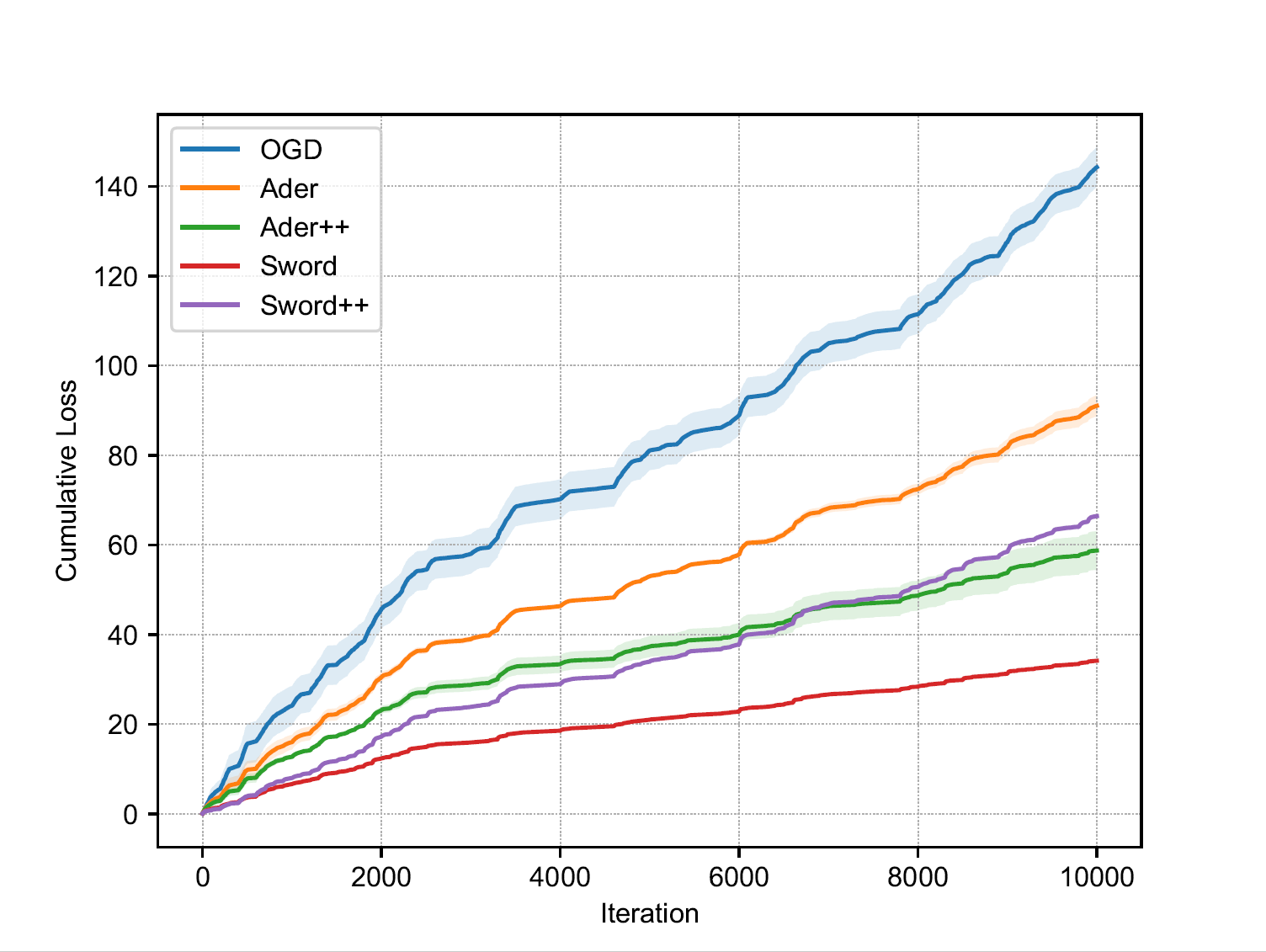 Figure(a): dynamic regret (full info) Figure(a): dynamic regret (full info) |
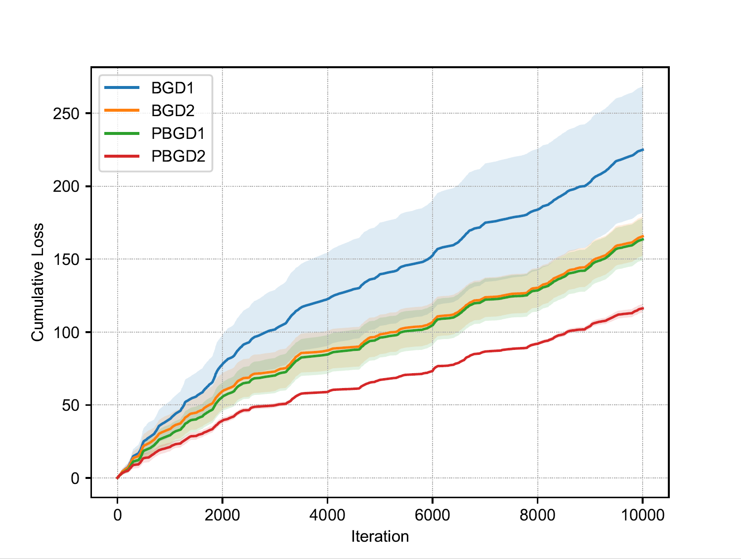 Figure(b): dynamic regret (bandit) Figure(b): dynamic regret (bandit) |
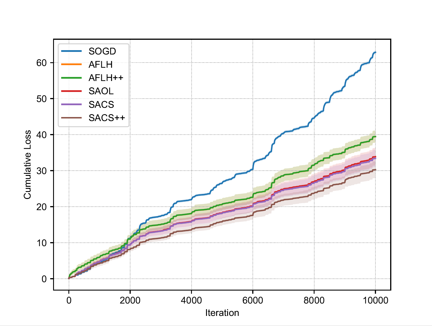 Figure(c): adaptive regret Figure(c): adaptive regret |
Similarly, we can run examples/bandit_dynamic and examples/adaptive
and get the results as shown in figure(b) and figure(c) for dynamic
algorithms with bandit information and adaptive algorithms with
full-information feedback, respectively. Note that it is proved that
designing strongly adaptive algorithms for bandit learning is impossible
Define user’s own algorithms
Finally, we use Ader and Ader++ as an example to illustrate how
to define meta-based structure algorithm based on our package.
Accept parameters as follows, where
domainis the feasible set,Tis the number of total rounds,Gis the upper bound of gradient,surrogatespecifies whether to use surrogate loss,min_step_sizeandmax_step_sizespecifies the range of step size pool, which are not necessary and will be set as the theory suggests if not given by the user.priorandseedspecify the initial decision of the model.from pynol.learner.models.model import Model class Ader(Model): def __init__(self, domain, T, G, surrogate=True, min_step_size=None, max_step_size=None, prior=None, seed=None):
Discrete the range of optimal step size to produce a candidate step size pool and return a bunch of base learners, each associated with a specific step size in the step size pool by
DiscretizedSSP.from pynol.learner.base import OGD from pynol.learner.schedule.ssp import DiscretizedSSP D = 2 * domain.R if min_step_size is None: min_step_size = D / G * (7 / (2 * T))**0.5 if max_step_size is None: max_step_size = D / G * (7 / (2 * T) + 2)**0.5 base_learners = DiscretizedSSP(OGD, min_step_size, max_step_size, grid=2, domain=domain, prior=prior, seed=seed)
Pass the base learners to
schedule.from pynol.learner.schedule.schedule import Schedule schedule = Schedule(base_learners)
Define meta algorithm by
meta.from pynol.learner.meta import Hedge from pynol.environment.domain import Simplex prob = Simplex(dimension=len(base_learners)).init(prior='nonuniform') lr = np.array([1 / (G * D * (t + 1)**0.5) for t in range(T)]) meta = Hedge(prob=prob, lr=lr)
Define the surrogate loss for base learners and meta learner by
specification.from pynol.learner.specification.surrogate_base import LinearSurrogateBase from pynol.learner.specification.surrogate_meta import SurrogateMetaFromBase if surrogate is False: surrogate_base, surrogate_meta = None, None # for Ader else: surrogate_base = LinearSurrogateBases() # for Ader++ surrogate_meta = SurrogateMetaFromBase()
Instantiate model by inheriting from
Modelclass and passingschedule,meta,specificationto initialize.super().__init__(schedule, meta, surrogate_base=surrogate_base, surrogate_meta=surrogate_meta)
Now, we finish the definition of Ader and Ader++. See more model
definition examples in models .