pynol.learner

base

This module provides different base algorithms. On the one hand, they can be used to optimize static regret directly, on the other hand, they are crucial components for algorithms designed to optimize dynamic regret and adaptive regret.

Base

class pynol.learner.base.Base(domain: Domain, step_size: float | ndarray, prior: list | ndarray | None = None, seed: int | None = None)

Bases: ABC

An abstract class for base algorithms.

Parameters:

• domain (Domain) – Feasible set for the base algorithm. step_size (float, numpy.ndarray): Step size \(\eta\) for the base algorithm. Valid types include float and numpy.ndarray. If the type of the step size \(\eta\) is float, the algorithm will use the fixed step size all the time, otherwise, the algorithm will use the step size \(\eta_t\) at round $t$.

• prior (str, numpy.ndarray, optional) – The initial decision of the algorithm is set as domain.init_x(prior, seed).

• seed (int, optional) – The initial decision of the algorithm is set as domain.init_x(prior, seed).

get_step_size()

Get the step size at each round.

Returns:

Step size at the current round.

Return type:

float

opt(env: Environment)

The optimization process of the base algorithm.

All base algorithms are divided into two parts: opt_by_optimism() at the beginning of current round and opt_by_gradient() at the end of current round.

Parameters:

env (Environment) – Environment at the current round.

Returns:

tuple contains:

x (numpy.ndarray): Decision at the current round.

loss (float): Origin loss at the current round.

surrogate_loss (float): the surrogate loss at the current round.

Return type:

tuple

abstract opt_by_gradient(env: Environment)

Optimize by the true gradient.

All base-algorithms are required to override this method to implement their own optimization process.

Parameters:

env (Environment) – Environment at the current round.

Returns:

tuple contains:

x (numpy.ndarray): the decision at the current round.

loss (float): the origin loss at the current round.

surrogate_loss (float): the surrogate loss at the current round.

Return type:

tuple

opt_by_optimism(optimism: ndarray | None = None)

Optimize by the optimism.

Parameters:

optimism (numpy.ndarray, optional) – External optimism at the beginning of the current round.

Returns:

None

reinit()

Reset the base algorithm to the initial state, which is used for adaptive algorithms.

OGD

class pynol.learner.base.OGD(domain: Domain, step_size: float | ndarray, prior: list | ndarray | None = None, seed: int | None = None)

Bases: Base

Implementation of Online Gradient Descent.

OGD stands for Online Gradient Descent, the most popular algorithm for online learning. OGD updates the decision \(x_{t+1}\) by

\[x_{t+1} = \Pi_{\mathcal{X}} [x_t - \eta_t \nabla f_t(x_t)]\]

where \(\eta_t > 0\) is the step size at round t, and \(\Pi_{\mathcal{X}}[\cdot]\) denotes the projection onto the nearest point in \(\mathcal{X}\).

Parameters:

• domain (Domain) – Feasible set for the base algorithm.

• step_size (float, numpy.ndarray) – Step size \(\eta\) for the base algorithm. Valid types include float and numpy.ndarray. If the type of the step size \(\eta\) is float, the algorithm will use the fixed step size all the time, otherwise, the algorithm will use the step size \(\eta_t\) at round $t$.

• prior (str, numpy.ndarray, optional) – The initial decision of the algorithm is set as domain.init_x(prior, seed).

• seed (int, optional) – The initial decision of the algorithm is set as domain.init_x(prior, seed).

opt_by_gradient(env: Environment)

Optimize by the true gradient.

All base-algorithms are required to override this method to implement their own optimization process.

Parameters:

env (Environment) – Environment at the current round.

Returns:

tuple contains:

x (numpy.ndarray): the decision at the current round.

loss (float): the origin loss at the current round.

surrogate_loss (float): the surrogate loss at the current round.

Return type:

tuple

BGDOnePoint

class pynol.learner.base.BGDOnePoint(domain: Domain, step_size: float | ndarray, scale_perturb: float, prior: list | ndarray | None = None, seed: int | None = None)

Bases: Base

Implementation of Bandit Convex Optimization with one-point feedback.

BGDOnePoint stands for Bandit Convex Optimization with one-point feedback, in which at each round the learner submits one decision and then can only observe the function value of this point. BGDOnePoint updates the decision \(x_{t+1}\) by

\[x_{t+1} = \Pi_{\mathcal{X}}[x_t - \eta_t \tilde{g}_t] \mbox{ with } \tilde{g}_t = \frac{d}{\delta}f_t(x_t + \delta s_t) \cdot s_t,\]

where \(\eta_t > 0\) is the step size at round t, \(d\) is the dimension, \(\delta\) is the scale of the perturbation, \(s_t\) is the unit vector selected uniformly at random and \(\Pi_{\mathcal{X}}[\cdot]\) denotes the projection onto the nearest point in \(\mathcal{X}\).

Parameters:

• domain (Domain) – Feasible set for the base algorithm.

• step_size (float, numpy.ndarray) – Step size \(\eta\) for the base algorithm. Valid types include float and numpy.ndarray. If the type of the step size \(\eta\) is float, the algorithm will use the fixed step size all the time, otherwise, the algorithm will use the step size \(\eta_t\) at round $t$.

• scale_perturb (float) – Scale of perturbation \(\delta\).

• prior (str, numpy.ndarray, optional) – The initial decision of the algorithm is set as domain.init_x(prior, seed).

• seed (int, optional) – The initial decision of the algorithm is set as domain.init_x(prior, seed).

References

https://arxiv.org/abs/cs/0408007

get_grad(dimension, loss, unit_vec) → ndarray

Estimate the gradient by \(\tilde{g}_t = \frac{d}{\delta}f_t(x_t + \delta s_t) \cdot s_t\).

Parameters:

• dimension (int) – Dimension of the decision.

• loss (float) – Loss of the submitted decision.

• unit_vec (numpy.ndarray) – Unit vector used to perturb the decision.

Returns:

the estimated gradient at the current round.

Return type:

numpy.ndarray

opt_by_gradient(env: Environment)

Optimize by the estimated gradient.

Parameters:

env (Environment) – Environment at the current round.

Returns:

tuple contains:

x (numpy.ndarray): Decision at the current round.

loss (float): the origin loss at the current round.

surrogate_loss (float): Surrogate loss at the current round.

Return type:

tuple

reinit()

Reset the base algorithm to the initial state, which is used for adaptive algorithms.

BGDTwoPoint

class pynol.learner.base.BGDTwoPoint(domain: Domain, step_size: float | list, scale_perturb: float, prior: list | ndarray | None = None, seed: int | None = None)

Bases: Base

Implementation of Bandit Convex Optimization with Two-point Feedback.

BGDTwoPoint stands for Bandit Convex Optimization with two-point feedback, in which at each round the learner submits two decisions and then can only observe the function values of these two points. BGDTwoPoint updates the decision \(x_{t+1}\) by

\[x_{t+1} = \Pi_{\mathcal{X}} [x_t - \eta_t \tilde{g}_t] \mbox{ with } \tilde{g}_t = \frac{d}{2\delta}(f_t(x_t + \delta s_t) - f_t(x_t - \delta s_t))\cdot s_t,\]

where \(\eta_t > 0\) is the step size at round t, \(d\) is the dimension, \(\delta\) is the scale of the perturbation, \(s_t\) is the unit vector selected uniformly at random, and \(\Pi_{\mathcal{X}}[\cdot]\) denotes the projection onto the nearest point in \(\mathcal{X}\).

Parameters:

• domain (Domain) – Feasible set for the base algorithm.

• step_size (float, numpy.ndarray) – Step size \(\eta\) for the base algorithm. Valid types include float and numpy.ndarray. If the type of the step size \(\eta\) is float, the algorithm will use the fixed step size all the time, otherwise, the algorithm will use the step size \(\eta_t\) at round $t$.

• scale_perturb (float) – Scale of perturbation \(\delta\).

• prior (str, numpy.ndarray, optional) – The initial decision of the algorithm is set as domain.init_x(prior, seed).

• seed (int, optional) – The initial decision of the algorithm is set as domain.init_x(prior, seed).

References

https://alekhagarwal.net/bandits-colt.pdf

get_grad(dimension, loss1, loss2, unit_vec)

Estimate the gradient by \(\tilde{g}_t = \frac{d}{2\delta}(f_t(x_t + \delta s_t) - f_t(x_t - \delta s_t))\cdot s_t\).

Parameters:

• dimension (int) – Dimension of the decision.

• loss1 (float) – Loss of the first submitted decision.

• loss2 (float) – Loss of the second submitted decision.

• unit_vec (numpy.ndarray) – Unit vector used to perturb the decision.

Returns:

Estimated gradient at the current round.

Return type:

numpy.ndarray

opt_by_gradient(env: Environment)

Optimize by the estimated gradient.

Parameters:

env (Environment) – Environment at the current round.

Returns:

tuple contains:

x (numpy.ndarray): Average decision at the current round.

loss (float): Average origin loss at the current round.

surrogate_loss (float): Average surrogate loss at the current round.

Return type:

tuple

reinit()

Reset the base algorithm to the initial state, which is used for adaptive algorithms.

SOGD

class pynol.learner.base.SOGD(domain: Domain, prior: list | ndarray | None = None, seed: int | None = None)

Bases: Base

Implementation of scale-free online learning.

SOGD stands for Scale-free Online Gradient Descent, an online convex optimization algorithm that achieves parameter-free and scale-free simultaneously, which is useful in deriving small-loss bound for smooth functions. SOGD updates the decision \(x_{t+1}\) by

\[x_{t+1} = \Pi_{\mathcal{X}}[x_t - \frac{1}{\sqrt{\delta + \sum_{s=1}^{t-1} \nabla f_s(x_s)}} \nabla f_t(x_t)]\]

where \(\delta\) is a small constant to avoid divide by \(0\), and \(\Pi_{\mathcal{X}}[\cdot]\) denotes the projection onto the nearest point in \(\mathcal{X}\). We set \(\delta=1\) in our implementation.

Parameters:

• domain (Domain) – Feasible set for the base algorithm.

• prior (str, numpy.ndarray, optional) – The initial decision of the algorithm is set as domain.init_x(prior, seed).

• seed (int, optional) – The initial decision of the algorithm is set as domain.init_x(prior, seed).

References

https://arxiv.org/abs/1601.01974

opt_by_gradient(env: Environment)

Optimize by the true gradient.

All base-algorithms are required to override this method to implement their own optimization process.

Parameters:

env (Environment) – Environment at the current round.

Returns:

tuple contains:

x (numpy.ndarray): the decision at the current round.

loss (float): the origin loss at the current round.

surrogate_loss (float): the surrogate loss at the current round.

Return type:

tuple

reinit()

Reset the base algorithm to the initial state, which is used for adaptive algorithms.

OptimisticBase

class pynol.learner.base.OptimisticBase(domain: Domain, step_size: float | list, optimism_type: str = 'external', prior: list | ndarray | None = None, seed: int | None = None)

Bases: Base

An abstract class for optimistic-type base algorithms.

The optimistic-type algorithms are very general and useful, and they can achieve a tighter regret guarantee with benign “predictable sequences”. There are mainly two types of optimistic algorithms: Optimistic Online Mirror Descent (Optimistic OMD) and Optimistic Follow The Regularized Leader (Optimistic FTRL). The general update rule of Optimistic OMD is as follows,

\[ \begin{align}\begin{aligned}x_t = {\arg\min}_{x \in \mathcal{X}} \ \eta_t \langle m_t, x\rangle + D_R(x, \hat{x}_t)\\\hat{x}_{t+1} = {\arg\min}_{x \in \mathcal{X}} \ \eta_t \langle \nabla f_t(x_t), x\rangle + D_R(x, \hat{x}_t),\end{aligned}\end{align} \]

and the general update rule of Optimistic FTRL is as follows,

\[x_t = {\arg\min}_{x \in \mathcal{X}} \ \eta_t \langle \sum_{s=1}^{t-1} \nabla f_s(x_s) + m_t, x\rangle + R(x),\]

where \(\eta_t\) is the step size at round \(t\), \(m_t\) is the optimism at the beginning of round \(t\), serving as a guess of the true gradient \(\nabla f_t(x_t)\) at round \(t\), \(R\) is the regularizer and \(D_R(\cdot, \cdot)\) is the Bregman divergence with respect to the regularizer \(R\).

Parameters:

• domain (Domain) – Feasible set for the base algorithm.

• step_size (float, numpy.ndarray) – Step size \(\eta\) for the base algorithm. Valid types include float and numpy.ndarray. If the type of the step size \(\eta\) is float, the algorithm will use the fixed step size all the time, otherwise, the algorithm will use the step size \(\eta_t\) at round \(t\).

• optimism_type (str, optional) – Type of optimism used for algorithm. Valid actions include external, last_grad, middle_grad and None. if optimism_type='external', the algorithm will accept the external specified \(m_t\) by the environment at each round; if optimism_type='last_grad', the optimism is set as \(m_t = \nabla f_{t-1}(x_{t-1})\); if optimism_type='middle_grad', the optimism is set as \(m_t = \nabla f_{t-1}(\hat{x}_t)\), and if optimism_type=None, the optimism is set as \(m_t = 0\).

• prior (str, numpy.ndarray, optional) – The initial decision of the algorithm is set as domain.init_x(prior, seed).

• seed (int, optional) – The initial decision of the algorithm is set as domain.init_x(prior, seed).

References

https://proceedings.mlr.press/v23/chiang12.html

compute_internal_optimism(env: Environment)

Compute the internal optimism.

Parameters:

env (Environment) – Environment at the current round.

reinit()

Reset the base algorithm to the initial state, which is used for adaptive algorithms.

OptimisticOGD

class pynol.learner.base.OptimisticOGD(domain: Domain, step_size: float | list, optimism_type: str = 'external', prior: list | ndarray | None = None, seed: int | None = None)

Bases: OptimisticBase

Implementation of Optimistic Online Gradient Descent.

OptimisticOGD is an online convex optimization algorithm, which is a specialization of Optimistic OMD with the Euclidean distance as the regularizer. OptimisticOGD updates the decision \(x_{t}\) by

\[ \begin{align}\begin{aligned}x_t = \Pi_{\mathcal{X}}[\hat{x}_t - \eta_t m_t]\\\hat{x}_{t+1} = \Pi_{\mathcal{X}}[\hat{x}_t - \eta_t \nabla f_t(x_t)],\end{aligned}\end{align} \]

where \(\eta_t > 0\) is the step size at round \(t\), \(m_t\) is the optimism at the beginning of round \(t\), and \(\Pi_{\mathcal{X}}[\cdot]\) denotes the projection onto the nearest point in \(\mathcal{X}\).

Parameters:

• domain (Domain) – Feasible set for the base algorithm.

• step_size (float, numpy.ndarray) – Step size \(\eta\) for the base algorithm. Valid types include float and numpy.ndarray. If the type of the step size \(\eta\) is float, the algorithm will use the fixed step size all the time, otherwise, the algorithm will use the step size \(\eta_t\) at round \(t\).

• optimism_type (str, optional) – Type of optimism used for algorithm. Valid actions include external, last_grad, middle_grad and None. if optimism_type='external', the algorithm will accept the external specified \(m_t\) by the environment at each round; if optimism_type='last_grad', the optimism is set as \(m_t = \nabla f_{t-1}(x_{t-1})\); if optimism_type='middle_grad', the optimism is set as \(m_t = \nabla f_{t-1}(\hat{x}_t)\), and if optimism_type=None, the optimism is set as \(m_t = 0\).

• prior (str, numpy.ndarray, optional) – The initial decision of the algorithm is set as domain.init_x(prior, seed).

• seed (int, optional) – The initial decision of the algorithm is set as domain.init_x(prior, seed).

Note

1. OGD is a special case of OptimisticOGD with optimism_type=None.

2. OEGD is a special case of OptimisticOGD with optimism_type='middle_grad.

References

https://proceedings.mlr.press/v30/Rakhlin13.html

opt_by_gradient(env: Environment)

Optimize by the true gradient.

All base-algorithms are required to override this method to implement their own optimization process.

Parameters:

env (Environment) – Environment at the current round.

Returns:

tuple contains:

x (numpy.ndarray): the decision at the current round.

loss (float): the origin loss at the current round.

surrogate_loss (float): the surrogate loss at the current round.

Return type:

tuple

opt_by_optimism(optimism: ndarray | None = None)

Optimize by the optimism.

Parameters:

optimism (numpy.ndarray, optional) – External optimism at the beginning of the current round.

Returns:

None

OEGD

class pynol.learner.base.OEGD(domain: Domain, step_size: float | ndarray, prior: list | ndarray | None = None, seed: int | None = None)

Bases: Base

Implementation of online extra-gradient descent.

OEGD stands for Online Extra-Gradient Descent. It is shown to enjoy gradient-variation regret guarantee, which would be smaller when the environments evolve gradually. OEGD updates decision \(x_t\) by

\[ \begin{align}\begin{aligned}x_t = \Pi_{\mathcal{X}}[\hat{x}_t - \eta_t \nabla f_{t-1}(\hat{x}_t)],\\\hat{x}_{t+1} = \Pi_{\mathcal{X}}[\hat{x}_t - \eta_t \nabla f_t(x_t)],\end{aligned}\end{align} \]

where \(\eta_t > 0\) is is the step size at round \(t\), and \(\Pi_{\mathcal{X}}[\cdot]\) denotes the projection onto the nearest point in \(\mathcal{X}\).

Parameters:

• domain (Domain) – Feasible set for the base algorithm.

• step_size (float, numpy.ndarray) – Step size \(\eta\) for the base algorithm. Valid types include float and numpy.ndarray. If the type of the step size \(\eta\) is float, the algorithm will use the fixed step size all the time, otherwise, the algorithm will use the step size \(\eta_t\) at round $t$.

• prior (str, numpy.ndarray, optional) – The initial decision of the algorithm is set as domain.init_x(prior, seed).

• seed (int, optional) – The initial decision of the algorithm is set as domain.init_x(prior, seed).

References

https://proceedings.mlr.press/v23/chiang12.html

opt_by_gradient(env: Environment)

Optimize by the true gradient.

All base-algorithms are required to override this method to implement their own optimization process.

Parameters:

env (Environment) – Environment at the current round.

Returns:

tuple contains:

x (numpy.ndarray): the decision at the current round.

loss (float): the origin loss at the current round.

surrogate_loss (float): the surrogate loss at the current round.

Return type:

tuple

opt_by_optimism(optimism: ndarray | None = None)

Optimize by the optimism.

Parameters:

optimism (numpy.ndarray, optional) – External optimism at the beginning of the current round.

Returns:

None

Hedge

class pynol.learner.base.Hedge(domain: Domain, step_size: float | list, is_lazy: bool = False, correct: bool = False, prior: list | ndarray | None = None, seed: int | None = None)

Bases: OptimisticHedge

Implementation of Hedge.

Hedge is the most popular algorithm for tracking the best expert problem. There are two versions of Hedge: the greedy version and the lazy version. The greedy version is a special case of Optimistic OMD with the negative entropy as the regularizer and optimism_type=None and the lazy version is a special case of Optimistic FTRL with the negative entropy as the regularizer and optimism_type=None. The greedy version Hedge updates the decision \(x_{t+1}\) by

\[x_{t+1} = \Pi_{\mathcal{X}}[x_t\exp(-\eta_t (\nabla f_t({x}_t) +a_t))],\]

and the lazy version Hedge updates the decision \(x_{t+1}\) by

\[x_{t+1} = \Pi_{\mathcal{X}}[x_1 \exp(-\eta_t (\sum_{s=1}^{t} (\nabla f_s(x_s) +a_s)))],\]

where \(\eta_t > 0\) is the step size, \(a_t\) is the correction term at round \(t\), and \(\Pi_{\mathcal{X}}[\cdot]\) denotes the projection onto the nearest point in \(\mathcal{X}\).

Parameters:

• domain (Domain) – Feasible set for the base algorithm.

• step_size (float, numpy.ndarray) – the step size \(\eta\) for the base algorithm. Valid types include float and numpy.ndarray. If the type of the step size \(\eta\) is float, the algorithm will use the fixed step size all the time, otherwise, the algorithm will use the step size \(\eta_t\) at round \(t\).

• is_lazy (bool) – Type of the update version: lazy or greedy. The default is False.

• correct (bool) – Whether to use correction term. \(a_t\) is set as \(a_t = \nabla f_t(x_t)^2\) if correct=True and \(a_t=0\) otherwise. The default is False.

• prior (str, numpy.ndarray, optional) – The initial decision of the algorithm is set as domain.init_x(prior, seed).

• seed (int, optional) – The initial decision of the algorithm is set as domain.init_x(prior, seed).

OptimisticHedge

class pynol.learner.base.OptimisticHedge(domain: Domain, step_size: float | list, optimism_type: str = 'external', is_lazy: bool = False, correct: bool = False, prior: list | ndarray | None = None, seed: int | None = None)

Bases: OptimisticBase

Implementation of Optimistic Hedge.

Hedge is the most popular algorithm for tracking the best expert problem. Optimistic Hedge is an enhanced version of Hedge which can further incorporate the knowledge of predictable sequences. There are two versions of Optimistic Hedge: the greedy version and the lazy version. The greedy version is a special case of Optimistic OMD with the negative entropy as the regularizer and the lazy version is a special case of Optimistic FTRL. The greedy version Optimistic Hedge updates the decision \(x_t\) by

\[ \begin{align}\begin{aligned}{x}_t = \Pi_{\mathcal{X}}[\hat{x}_{t} \exp(-\eta_t m_{t})]\\\hat{x}_{t+1} = \Pi_{\mathcal{X}}[\hat{x}_t\exp(-\eta_t (\nabla f_t({x}_t) +a_t))],\end{aligned}\end{align} \]

and the lazy version Optimistic Hedge updates the decision \(x_t\) by

\[x_t = \Pi_{\mathcal{X}}[x_1 \exp(-\eta_t (\sum_{s=1}^{t-1} (\nabla f_s(x_s) +a_s) + m_t))],\]

where \(\eta_t > 0\) is the step size at round \(t\), \(m_t\) is the optimism at the beginning of round \(t\), \(a_t\) is the correction term and \(\Pi_{\mathcal{X}}[\cdot]\) denotes the projection onto the nearest point in \(\mathcal{X}\).

Parameters:

• domain (Domain) – Feasible set for the base algorithm.

• step_size (float, numpy.ndarray) – Step size \(\eta\) for the base algorithm. Valid types include float and numpy.ndarray. If the type of the step size \(\eta\) is float, the algorithm will use the fixed step size all the time, otherwise, the algorithm will use the step size \(\eta_t\) at round \(t\).

• optimism_type (str, optional) – Type of optimism used for algorithm. Valid actions include external, last_grad, middle_grad and None. if optimism_type='external', the algorithm will accept the external specified \(m_t\) by the environment at each round; if optimism_type='last_grad', the optimism is set as \(m_t = \nabla f_{t-1}(x_{t-1})\); if optimism_type='middle_grad', the optimism is set as \(m_t = \nabla f_{t-1}(\hat{x}_t)\), and if optimism_type=None, the optimism is set as \(m_t = 0\).

• is_lazy (bool) – Type of the update version: lazy or greedy. The default is False.

• correct (bool) – Whether to use correction term. \(a_t\) is set as \(a_t = \eta_t (\nabla f_t(x_t) - m_t)^2\) if correct=True and \(a_t=0\) otherwise. The default is False.

• prior (str, numpy.ndarray, optional) – The initial decision of the algorithm is set as domain.init_x(prior, seed).

• seed (int, optional) – The initial decision of the algorithm is set as domain.init_x(prior, seed).

References

http://proceedings.mlr.press/v30/Rakhlin13.pdf

Note

1. Greedy version Optimistic Hedge is a special case of OptimisticOMD with the negative entropy as the regularizer.

2. Lazy version Optimistic Hedge is a special case of OptimisticFTRL with the negative entropy as the regularizer.

opt_by_gradient(env: Environment)

Optimize by the true gradient.

All base-algorithms are required to override this method to implement their own optimization process.

Parameters:

env (Environment) – Environment at the current round.

Returns:

tuple contains:

x (numpy.ndarray): the decision at the current round.

loss (float): the origin loss at the current round.

surrogate_loss (float): the surrogate loss at the current round.

Return type:

tuple

opt_by_optimism(optimism: ndarray | None = None)

Optimize by the optimism.

Parameters:

optimism (numpy.ndarray, optional) – External optimism at the beginning of the current round.

Returns:

None

reinit()

Reset the base algorithm to the initial state, which is used for adaptive algorithms.

meta

This module provides different meta algorithms. On the one hand, they can be used to solve the expert-tracking problem directly, on the other hand, they are crucial components to combine the base-learners to optimize dynamic regret and adaptive regret.

Meta

class pynol.learner.meta.Meta(prob: ndarray, lr: float | ndarray | OptimisticLR)

Bases: ABC

An abstract class for meta-algorithms.

Parameters:

• prob (numpy.ndarray) – Initial probability over the base-learners.

• lr (float, numpy.ndarray, OptimisticLR) – Learning rate for meta-algorithm.

property active_state

Get the active state of base-learners:

• 0: sleep

• 1: active at the current round and the previous round.

• 2: active at the current round and sleep at the previous round.

get_lr()

Compute the learning rate for meta-algorithms.

If the type of the learning rate \(\varepsilon\) is float, this method will return the constant learning rate \(\varepsilon\) all the time; if the type of \(\varepsilon\) is numpy.ndarray with shape [T, ], this method will return a scalar \(\varepsilon[t]\) at round \(t\); if the type of \(\varepsilon\) is numpy.ndarray with shape [T, N] where \(N\) is the dimension, this method will return a vector \(\varepsilon[t]\) at time \(t\); if the type of \(\varepsilon\) is numpy.ndarray with shape [1, N], this method will return a vector \(\varepsilon\) all the time; if the type of \(\varepsilon\) is OptimisticLR(), the learning rate \(\varepsilon_t\) is computed by compute_lr() at round \(t\).

property init_prob

Get the initial probability over the current alive base-learners.

opt(loss_bases: ndarray, loss_meta: float | None = None, optimism: ndarray | None = None)

The optimization process of the meta-algorithm.

All base algorithms are divided into two parts: opt_by_optimism() at the beginning of current round and opt_by_gradient() at the end of current round.

Parameters:

• loss_bases (numpy.ndarray) – Losses of all alive base-learners.

• loss_meta (float, optional) – Loss of the combined decision.

• optimism (numpy.ndarray) – Optimism at the beginning of the current round, serving as a guess of loss_bases.

Returns:

Probability over the alive base-learners.

Return type:

numpy.ndarray

abstract opt_by_gradient(loss_bases: ndarray, loss_meta: float | None = None)

Optimize by the true gradient (loss).

All base-algorithms are required to override this method to implement their own optimization process.

Parameters:

• loss_bases (numpy.ndarray) – Losses of all alive base-learners.

• loss_meta (float) – Loss of the combined decision.

Returns:

Probability over the alive base-learners.

Return type:

numpy.ndarray

opt_by_optimism(optimism: ndarray | None)

Optimize by the optimism.

Parameters:

optimism (numpy.ndarray, optional) – the optimism at the beginning of the current round.

Returns:

None

property prob

Get the current probability over the alive base-learners.

Hedge

class pynol.learner.meta.Hedge(prob: ndarray, lr: float | ndarray | OptimisticLR, is_lazy: bool = False, correct: bool = False)

Bases: OptimisticHedge

Implementation of Hedge.

Hedge is the most popular algorithm for tracking the best expert problem. There are two versions of Hedge: the greedy version and the lazy version. The greedy version is a special case of Optimistic OMD with the negative entropy as the regularizer and optimism_type=None and the lazy version is a special case of Optimistic FTRL with the negative entropy as the regularizer and optimism_type=None. The greedy version Hedge updates the decision \(p_{t+1}\) by

\[p_{t+1, i} \propto p_{t,i} \exp \Big(-\varepsilon_t (\ell_{t,i} + b_{t,i}) \Big), \forall i \in [N],\]

and the lazy version Hedge updates the decision \(p_{t+1}\) by

\[p_{t+1, i} \propto p_{1,i} \exp \Big(-\varepsilon_t \sum_{s=1}^{t} (\ell_{s,i} + b_{s,i})\Big), \forall i \in [N],\]

where \(\varepsilon_t > 0\) is the step size, \(b_t\) is the correction term at round \(t\).

Parameters:

• prob (numpy.ndarray) – Initial probability over the base-learners.

• lr (float, numpy.ndarray, OptimisticLR) – The learning rate for meta-algorithm.

• is_lazy (bool) – Type of the update version: lazy or greedy. The default is False.

• correct (bool) – Whether to use correction term. \(b_t\) is set as \(b_t = \varepsilon_t \ell_t^2\) if correct=True and \(b_t=0\) otherwise. The default is False.

References

http://proceedings.mlr.press/v30/Rakhlin13.pdf

Note

1. Hedge is a special case of OptimisticHedge with optimism_type=None.

OptimisticMeta

class pynol.learner.meta.OptimisticMeta(prob: ndarray, lr: float | ndarray | OptimisticLR, optimism_type: str | None = 'external')

Bases: Meta

An abstract class for optimistic-type base algorithms.

The optimistic-type algorithms are very general and useful, and they can achieve a tighter regret guarantee with benign “predictable sequences”. There are mainly two types of optimistic algorithms: Optimistic Online Mirror Descent (Optimistic OMD) and Optimistic Follow The Regularized Leader (Optimistic FTRL). The general update rule of Optimistic OMD is as follows,

\[ \begin{align}\begin{aligned}p_t = {\arg\min}_{p \in \Delta_N} \ \varepsilon_t \langle M_t, p\rangle + D_R(p, \hat{p}_t)\\\hat{p}_{t+1} = {\arg\min}_{x \in \Delta_N} \ \varepsilon_t \langle \ell_t, p\rangle + D_R(p, \hat{p}_t),\end{aligned}\end{align} \]

and the general update rule of Optimistic FTRL is as follows,

\[p_t = {\arg\min}_{x \in \Delta_N} \ \varepsilon_t \langle \sum_{s=1}^{t-1} \ell_s + M_t, x\rangle + R(x),\]

where \(\varepsilon_t\) is the step size at round \(t\), \(M_t\) is the optimism at the beginning of round \(t\), serving as a guess of the true gradient \(\ell_t\) at round \(t\), \(R\) is the regularizer and \(D_R(\cdot, \cdot)\) is the Bregman divergence with respect to the regularizer \(R\).

Parameters:

• prob (numpy.ndarray) – The initial probability over the base-learners.

• lr (float, numpy.ndarray, OptimisticLR) – The learning rate for meta-algorithm.

• optimism_type (str, optional) – the type of optimism used for algorithm. Valid actions include external, last_loss and None. if optimism_type='external', the algorithm will accept the external optimism \(M_t\) at each round; if optimism_type='last_loss', the optimism is set as \(M_t = \ell_{t-1}\); and if optimism_type=None, the optimism is set as \(M_t = 0\).

References

https://proceedings.mlr.press/v23/chiang12.html

compute_internal_optimism(loss_bases: ndarray)

Compute the internal optimism for the next round.

If optimism_type='last_loss', the interval optimism is set as \(M_t = \ell_{t-1}\).

Parameters:

loss_bases (numpy.ndarray) – Losses of base-learners at the current round.

property middle_prob

Get the current intermediate probability over the alive base-learners.

property optimism

Get the current optimism of the alive base-learners.

OptimisticLR

class pynol.learner.meta.OptimisticLR(scale: float = 1.0, norm: int = inf, order: int = 2, upper_bound: float = 1.0)

Bases: object

An self-confident tuning method for optimistic algorithms.

The update rule of the optimistic learning rate is

\[\varepsilon_t = \frac{\alpha}{\sqrt{\sum_{s=1}^{t-1}\lVert \ell_t - M_t \rVert_p^q}},\]

where \(\alpha\) is the scale parameter, \(p\) is the norm order and :math`q` is the order.

Parameters:

• scale (float) – Scale parameter.

• norm (int, inf) – Order of norm \(p\).

• order (int) – Order of the norm value \(q\).

• upper_bound (float) – Upper bound of learning rate.

update_lr(optimism, loss)

Update learning rate by optimism and loss of the current round.

OptimisticHedge

class pynol.learner.meta.OptimisticHedge(prob: ndarray, lr: float | ndarray | OptimisticLR, optimism_type: str | None = 'external', is_lazy: bool = False, correct: bool = False)

Bases: OptimisticMeta

Implementation of Optimistic Hedge.

Hedge is the most popular algorithm for tracking the best expert problem. Optimistic Hedge is an enhanced version of Hedge which can further incorporate the knowledge of predictable sequences. There are two versions of Optimistic Hedge: the greedy version and the lazy version. The greedy version is a special case of Optimistic OMD with the negative entropy as the regularizer and the lazy version is a special case of Optimistic FTRL. The greedy version Optimistic Hedge updates the decision \(p_t\) by

\[ \begin{align}\begin{aligned}{p}_{t, i} = \frac{\hat{p}_{t,i}\exp(-\varepsilon_t M_{t,i})}{\sum_{j=1}^N \hat{p}_{t,j} \exp(-\varepsilon_t M_{t,j})}, \forall i \in [N]\\\hat{p}_{t+1, i} = \frac{\hat{p}_{t,i}\exp(-\varepsilon_t (\ell_{t,i} + b_{t,i}))}{\sum_{j=1}^N \hat{p}_{t,j} \exp(-\varepsilon_t (\ell_{t,j}+ b_{t,j}))}, \forall i \in [N],\end{aligned}\end{align} \]

and the lazy version Optimistic Hedge updates the decision \(x_t\) by

\[p_{t, i} \propto p_{1,i} \exp \Big(-\varepsilon_t (\sum_{s=1}^{t-1} (\ell_{s,i} + b_{s,i})+ m_{t,i})\Big), \forall i \in [N],\]

where \(\varepsilon_t > 0\) is the learning rate at round \(t\), \(M_t\) is the optimism at the beginning of round \(t\), \(b_t\) is the correction term.

Parameters:

• prob (numpy.ndarray) – Initial probability over the base-learners.

• lr (float, numpy.ndarray, OptimisticLR) – The learning rate for meta-algorithm.

• optimism_type (str, optional) – Type of optimism used for algorithm. Valid actions include external, last_loss and None. if optimism_type='external', the algorithm will accept the external optimism \(M_t\) at each round; if optimism_type='last_loss', the optimism is set as \(M_t = \ell_{t-1}\); and if optimism_type=None, the optimism is set as \(M_t = 0\).

• is_lazy (bool) – Type of the update version: lazy or greedy. The default is False.

• correct (bool) – Whether to use correction term. \(b_t\) is set as \(b_t = \varepsilon_t (\ell_t-M_t)^2\) if correct=True and \(b_t=0\) otherwise. The default is False.

Note

1. Greedy version Optimistic Hedge is a special case of OptimisticOMD with the negative entropy as the regularizer.

2. Lazy version Optimistic Hedge is a special case of OptimisticFTRL with the negative entropy as the regularizer.

property cum_loss

Get the cumulative loss of the alive base-learners.

opt_by_gradient(loss_bases: ndarray, loss_meta: float | None = None)

Optimize by the true gradient (loss).

All base-algorithms are required to override this method to implement their own optimization process.

Parameters:

• loss_bases (numpy.ndarray) – Losses of all alive base-learners.

• loss_meta (float) – Loss of the combined decision.

Returns:

Probability over the alive base-learners.

Return type:

numpy.ndarray

opt_by_optimism(optimism: ndarray | None)

Optimize by the optimism.

Parameters:

optimism (numpy.ndarray, optional) – the optimism at the beginning of the current round.

Returns:

None

MSMWC

class pynol.learner.meta.MSMWC(prob: ndarray, lr: float | ndarray | OptimisticLR, optimism_type: str | None = 'external')

Bases: OptimisticMeta

Implementation of Impossible Tuning Made Possible: A New Expert Algorithm and Its Applications.

MSMWC stands for Multi-scale Multiplicative-weight with Correction, a multi-scale expert-tracking algorithms that achieves second-order small-loss regret simultaneously for all expert. It can further exploit the knowledge of optimism to achieve tighter bound. The update rule of MSMWC is as follows,

\[ \begin{align}\begin{aligned}p_t = {\arg\min}_{p \in \Delta_N} \ \varepsilon_t \langle p, M_t\rangle + D_R(p, \hat{p}_t)\\\hat{p}_{t+1} = {\arg\min}_{p \in \Delta_N} \ \varepsilon_t \langle p, \ell_t + b_t\rangle + D_R(p, \hat{p}_t),\end{aligned}\end{align} \]

where \(\varepsilon_t > 0\) is the step size, \(b_t = \varepsilon_t (\ell_t - M_t)^2\) is the correction term at round \(t\), \(R\) is the weighted regularizer \(R(p) = \sum_{i=1}^N \frac{1}{\varepsilon_{t,i}}p_i \ln p_i\) and \(D_R(\cdot, \cdot)\) is the Bregman divergence with respect to the regularizer \(R\).

Parameters:

• prob (numpy.ndarray) – Initial probability over the base-learners.

• lr (float, numpy.ndarray, OptimisticLR) – The learning rate for meta-algorithm.

• optimism_type (str, optional) – Type of optimism used for algorithm. Valid actions include external, last_loss and None. if optimism_type='external', the algorithm will accept the external optimism \(M_t\) at each round; if optimism_type='last_loss', the optimism is set as \(M_t = \ell_{t-1}\); and if optimism_type=None, the optimism is set as \(M_t = 0\).

References

https://arxiv.org/abs/2102.01046

opt_by_gradient(loss_bases: ndarray, loss_meta: float | None = None)

Optimize by the true gradient (loss).

All base-algorithms are required to override this method to implement their own optimization process.

Parameters:

• loss_bases (numpy.ndarray) – Losses of all alive base-learners.

• loss_meta (float) – Loss of the combined decision.

Returns:

Probability over the alive base-learners.

Return type:

numpy.ndarray

opt_by_optimism(optimism: ndarray | None)

Optimize by the optimism.

Parameters:

optimism (numpy.ndarray, optional) – the optimism at the beginning of the current round.

Returns:

None

project(prob: ndarray, lr: ndarray)

Project \(p'\) back to the simplex by

\[p = {\arg\min}_{\Delta_N} \ D_R(p, p')\]

where \(R\) is the weighted regularizer \(R(p) = \sum_{i=1}^N \frac{1}{\varepsilon_{i}}p_i \ln p_i\) and \(D_R(\cdot, \cdot)\) is the Bregman divergence with respect to the regularizer \(R\).

Parameters:

• prob (numpy.ndarray) – Probability to be projected.

• lr (numpy.ndarray) – Learning rate of the weighted regularizer \(R\).

Prod

class pynol.learner.meta.Prod(N: int, lr: float | ndarray)

Bases: Meta

Implementation of Improved Second-Order Bounds for Prediction with Expert Advice and Strongly Adaptive Online Learning.

Prod can be view as a first-order approximation to weighted majority majority, which is proved to enjoy second-order bounds. The update rule is as follows:

\[p_{t+1,i} = (1+\varepsilon_{t,i}) p_{t,i} / W_{t+1},\]

where \(\varepsilon_t > 0\) is the learning rate and \(W_{t+1}\) is the normalization constant.

Parameters:

• N (int) – Number of the total base-learners.

• lr (float, numpy.ndarray) – Learning rate of meta-algorithm.

References

https://link.springer.com/content/pdf/10.1007/s10994-006-5001-7.pdf

http://proceedings.mlr.press/v37/daniely15.pdf

property active_state

Get the active state of base-learners:

• 0: sleep

• 1: active at the current round and the previous round.

• 2: active at the current round and sleep at the previous round.

opt_by_gradient(loss_bases, loss_meta)

Optimize by the true gradient (loss).

All base-algorithms are required to override this method to implement their own optimization process.

Parameters:

• loss_bases (numpy.ndarray) – Losses of all alive base-learners.

• loss_meta (float) – Loss of the combined decision.

Returns:

Probability over the alive base-learners.

Return type:

numpy.ndarray

AdaNormalHedge

class pynol.learner.meta.AdaNormalHedge(N: int)

Bases: Meta

Implementation of Achieving All with No Parameters: AdaNormalHedge.

AdaNormalHedge is a powerful parameter-free PEA algorithm that attains many interesting data-dependent bounds without any prior information. Notice that when using it as the meta-algorithm to combine base-learners, the input loss should be non-negative.

Parameters:

N (int) – Number of the total base-learners.

References

http://proceedings.mlr.press/v40/Luo15.pdf

property active_state

Get the active state of base-learners:

• 0: sleep

• 1: active at the current round and the previous round.

• 2: active at the current round and sleep at the previous round.

opt_by_gradient(loss_bases, loss_meta)

Optimize by the true gradient (loss).

All base-algorithms are required to override this method to implement their own optimization process.

Parameters:

• loss_bases (numpy.ndarray) – Losses of all alive base-learners.

• loss_meta (float) – Loss of the combined decision.

Returns:

Probability over the alive base-learners.

Return type:

numpy.ndarray

AFLHMeta

class pynol.learner.meta.AFLHMeta(N: int, lr: float | ndarray)

Bases: Meta

Implementation of the meta-algorithm of Adaptive algorithms for online decision problems.

AdaNormalHedge is a powerful parameter-free PEA algorithm that attains many interesting data-dependent bounds without any prior information. Notice that when using it as the meta-algorithm to combine base-learners, the input loss should be non-negative.

Parameters:

• N (int) – Number of the total base-learners.

• lr (float, numpy.ndarray) – Learning rate for meta-algorithm.

References

https://dominoweb.draco.res.ibm.com/reports/rj10418.pdf

property active_state

Get the active state of base-learners:

• 0: sleep

• 1: active at the current round and the previous round.

• 2: active at the current round and sleep at the previous round.

opt_by_gradient(loss_bases, loss_meta)

Optimize by the true gradient (loss).

All base-algorithms are required to override this method to implement their own optimization process.

Parameters:

• loss_bases (numpy.ndarray) – Losses of all alive base-learners.

• loss_meta (float) – Loss of the combined decision.

Returns:

Probability over the alive base-learners.

Return type:

numpy.ndarray

schedule

pynol.learner.schedule is the component to deal with the non-stationary environments. This module consists of two main parts: SSP and Cover. SSP specifies how to initialize the base-learners, which is important for dynamic algorithms. The dynamic algorithms construct a step size pool at first, and then initialize multiple base-learners, each employs a specific step size. The construction is based on exponential discretization of possible range of the optimal step size that usually depends on unknown path-length. Cover contains different interval partitions (Cover) that base-learners will last for, such as data stream cover (DSC), geometric cover (GC), compact GC (CGC) and its problem-dependent version CPGC, which is important for adaptive algorithm.

SSP

SSP

class pynol.learner.schedule.ssp.SSP(bases: list | None = None)

Bases: object

The simplest class to initialize base-learners, which accepts the base instances as the input directly.

Parameters:

bases (list) – List of base-learners.

StepSizeFreeSSP

class pynol.learner.schedule.ssp.StepSizeFreeSSP(base_class: Base, num_bases: int, **kwargs_base: dict)

Bases: SSP

The class to initialize step size free base-learners.

Parameters:

• base_class (Base) – Base class to schedule.

• num_bases (int) – Number of base-learners.

• **kwargs_base (dict) – Parameters of base-learners.

DiscreteSSP

class pynol.learner.schedule.ssp.DiscreteSSP(base_class: Base, min_step_size: float, max_step_size: float, grid: int = 2, **kwargs_base)

Bases: SSP

The most commonly used SSP for dynamic algorithms, which construct a step size pool at first, and then initialize multiple base-learners, each employs a specific step size.

Parameters:

• base_class (Base) – Base class to initialize.

• min_step_size (float) – Minimal value of the possible range of the optimal step size.

• max_step_size (float) – Maximal value of the possible range of the optimal step size.

• grid (int) – Grid size to discretize the possible range of the optimal step size.

• **kwargs (dict) – Parameter of the base-learners.

static discretize(min_step_size: float, max_step_size: float, grid: float = 2.0)

Discretize the possible range of the optimal step size exponentially

Parameters:

• min_step_size (float) – Minimal value of the possible range of the optimal step size.

• max_step_size (float) – Maximal value of the possible range of the optimal step size.

• grid (int) – Grid size to discretize the possible range of the optimal step size.

Cover

Cover

class pynol.learner.schedule.cover.Cover(active_state: ndarray, alive_time_threshold: int | None = None)

Bases: ABC

The abstract class for problem-independent cover.

Parameters:

• active_state (numpy.ndarray) – Initial active state.

• alive_time_threshold (int, optional) – Minimal interval length for cover. All intervals whose length are less than alive_time_threshold will not be activated.

property active_state

Get the active state of base-learners:

• 0: sleep

• 1: active at the current round and the previous round.

• 2: active at the current round and sleep at the previous round.

check_threshold()

Check the interval length. All intervals whose length are less than alive_time_threshold will not be activated.

abstract property t

Set the number of current round and compute the active state at current round.

FullCover

class pynol.learner.schedule.cover.FullCover(N: int)

Bases: Cover

The cover that sets all base-learners alive all the time, which is used for dynamic algorithms.

Parameters:

N (int) – Number of base-learners.

property t

Set the number of current round and compute the active state at current round.

GC

class pynol.learner.schedule.cover.GC(N: int, alive_time_threshold: int | None = None)

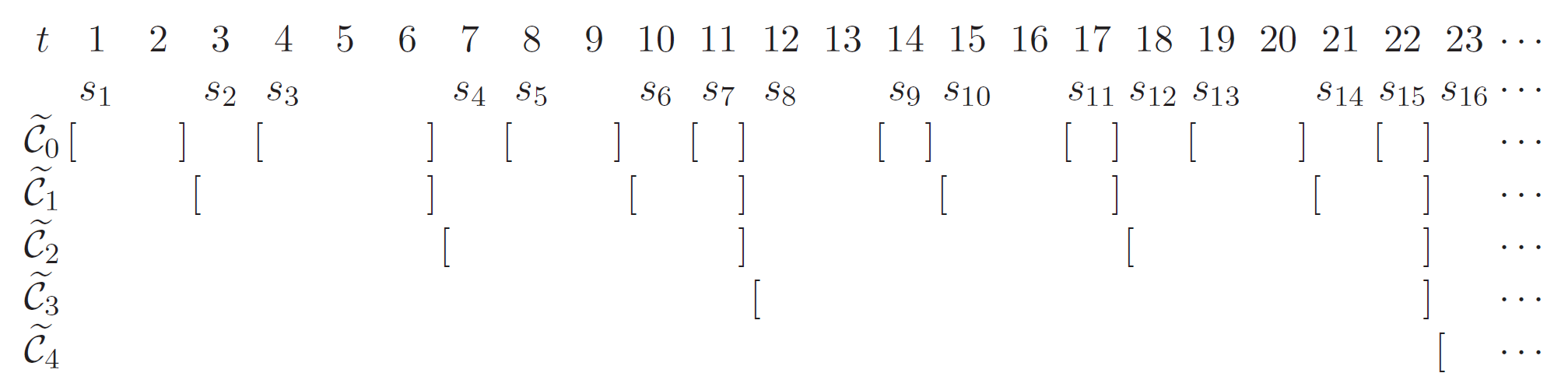
Bases: Cover

Geometric cover is the classical interval partition method, which discretize the whole horizon into sub-intervals with exponential length. Below is an illustration.

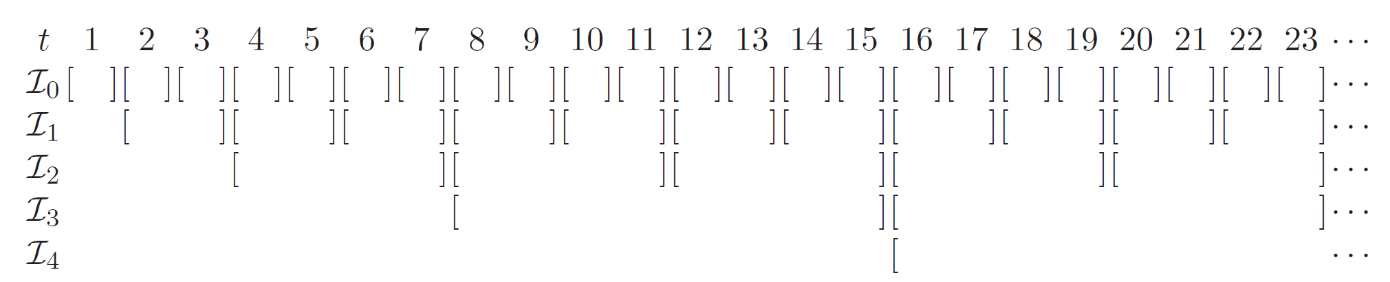
Parameters:

• N (int) – Number of base-learners. \(N=5\) for the above figure.

• alive_time_threshold (int, optional) – Minimal interval length for cover. All intervals whose length are less than alive_time_threshold will not be activated.

Below we give an example of GC with alive_time_threshold=4: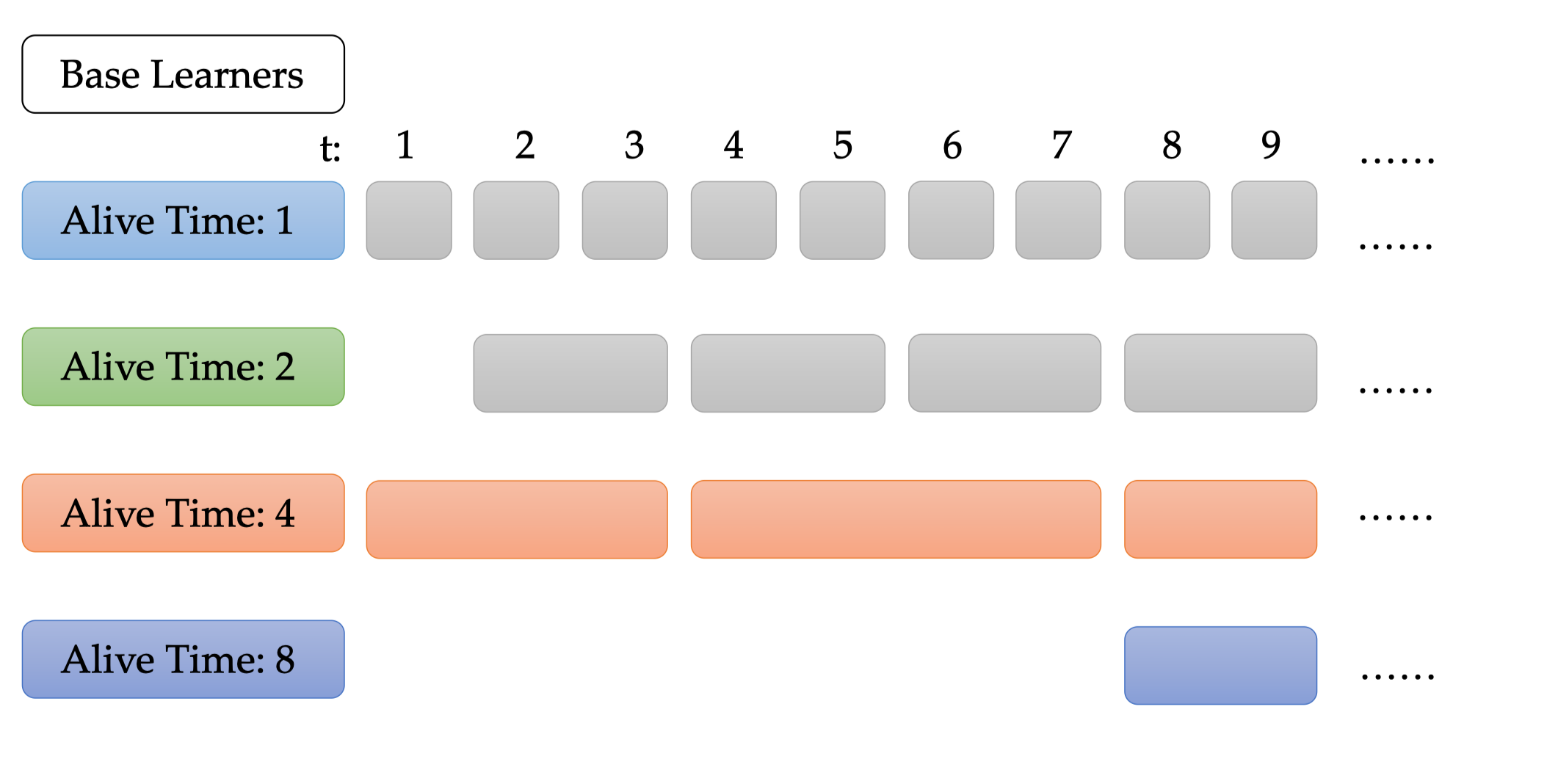

The base-learners whose alive time is less than 4 will not be activated, shown as gray blocks. Since there must be at least one base-learner, we initialize base-learner with Alive Time = 4 at t=1.

property t

Set the number of current round and compute the active state at current round.

CGC

class pynol.learner.schedule.cover.CGC(N: int, alive_time_threshold: int | None = None)

Bases: GC

CGC stands for compact geometric cover which removes some redundant intervals from geometric cover while keeping the desired properties. Below is an illustration.

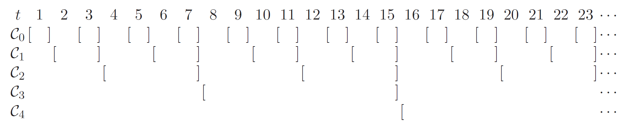
Parameters:

• N (int) – Number of base-learners. \(N=5\) for the above figure.

• alive_time_threshold (int, optional) – Minimal interval length for cover. All intervals whose length are less than alive_time_threshold will not be activated.

property t

Set the number of current round and compute the active state at current round.

PCover

class pynol.learner.schedule.cover.PCover(active_state: ndarray, loss_threshold: float = 2)

Bases: ABC

The abstract class for problem-dependent cover.

Parameters:

• active_state (numpy.ndarray) – Initial active state.

• loss_threshold (int, optional) – A new interval is activated only when the cumulative loss of the additional benchmark base-learner is larger than the loss_threshold.

property active_state

Get the active state of base-learners:

• 0: sleep

• 1: active at the current round and the previous round.

• 2: active at the current round and sleep at the previous round.

abstract set_instance_loss(loss: float)

Set the loss of the additional benchmark base-learner.

Parameters:

loss (float) – Loss of the additional benchmark base-learner.

Returns:

Whether to activate a new interval.

Return type:

bool

abstract property t

Set the number of current round and compute the active state at current round.

PGC

class pynol.learner.schedule.cover.PGC(N: int, loss_threshold: float = 2)

Bases: PCover

PGC stands for problem-dependent geometric cover, a problem-dependent version of geometric cover. Compared with geometric cover, it can achieve more adaptive results with proper base and meta-algorithms. Below is an illustration.

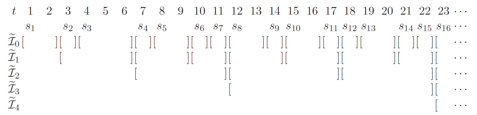
Parameters:

• active_state (numpy.ndarray) – Initial active state.

• loss_threshold (int, optional) – A new interval is activated only when the cumulative loss of the additional benchmark base-learner is larger than the loss_threshold.

set_instance_loss(loss: float)

Set the loss of the additional benchmark base-learner.

Parameters:

loss (float) – Loss of the additional benchmark base-learner.

Returns:

Whether to activate a new interval.

Return type:

bool

property t

Set the number of current round and compute the active state at current round.

PCGC

class pynol.learner.schedule.cover.PCGC(N: int, loss_threshold: float = 2)

Bases: PGC

PCGC stands for problem-dependent compact geometric cover which removes some redundant intervals from problem-dependent geometric cover while keeping the desired properties. Below is an illustration.

Parameters:

• active_state (numpy.ndarray) – Initial active state.

• loss_threshold (int, optional) – A new interval is activated only when the cumulative loss of the additional benchmark base-learner is larger than the loss_threshold.

property t

Set the number of current round and compute the active state at current round.

Schedule

Schedule

class pynol.learner.schedule.schedule.Schedule(ssp: SSP, cover: Cover | None = None)

Bases: object

The class to schedule base-learners with problem-independent cover.

Parameters:

• ssp (SSP) – A ssp instance containing a bunch of initialized base-learners.

• cover (Cover, optional) – A cover instance deciding the active state of base-learners.

opt_by_gradient(env: Environment)

Optimize by the gradient for all base-learners.

Parameters:

env (Environment) – Environment at current round.

Returns:

tuple contains:

loss (float): the origin loss of all alive base-learners.

surrogate_loss (float): the surrogate loss of all alive base-learners.

Return type:

tuple

opt_by_optimism(optimism: ndarray)

Optimize by the optimism for all base-learners.

Parameters:

optimism (numpy.ndarray) – External optimism for all alive base-learners.

property optimism

Get the optimisms of all alive base-learners.

Returns:

Optimisms of all alive base learners.

Return type:

numpy.ndarray

reinit_bases()

Reinitialize the base-learners whose active state is 2.

property t

Set the number of current round, get active state from cover and reinitialize the base-learners whose active state is 2.

property x_active_bases

Get the decisions of all alive base-learners.

Returns:

Decisions of all alive base learners.

Return type:

numpy.ndarray

PSchedule

class pynol.learner.schedule.schedule.PSchedule(ssp: SSP, cover: PCover | None = None)

Bases: Schedule

The class to schedule base-learners with problem-dependent cover.

Parameters:

• ssp (SSP) – A ssp instance containing a bunch of initialized base-learners.

• cover (PCover, optional) – A cover instance deciding the active state of base-learners.

opt_by_gradient(env)

Optimize by the gradient for all base-learners.

Parameters:

env (Environment) – Environment at current round.

Returns:

tuple contains:

loss (float): the origin loss of all alive base-learners.

surrogate_loss (float): the surrogate loss of all alive base-learners.

Return type:

tuple

opt_by_optimism(optimism: ndarray)

Optimize by the optimism for all base-learners.

Parameters:

optimism (numpy.ndarray) – External optimism for all alive base-learners.

property optimism

Get the optimisms of all alive base-learners.

Returns:

Optimisms of all alive base learners.

Return type:

numpy.ndarray

reinit_bases()

Reinitialize the base-learners whose active state is 2.

property t

Set the number of current round, get active state from cover and reinitialize the base-learners whose active state is 2.

property x_active_bases

Get the decisions of all alive base-learners.

Returns:

Decisions of all alive base learners.

Return type:

numpy.ndarray

specification

Besides Base, Meta and Schedule three main components, the remaining parts of algorithms are collectively referred to specification, which mainly includes the design of optimism and surrogate loss. As many algorithms can be viewed as specials cases of Optimistic Mirror Descent, the construction of optimism is crucial in algorithmic design. Moreover, replacing original loss function by surrogate loss is a useful technique which can bring great benefits sometimes.

SurrogateBase

SurrogateBase

class pynol.learner.specification.surrogate_base.SurrogateBase

Bases: ABC

The abstract class defines the surrogate loss functions and surrogate gradient (if possible) for base-learners.

abstract compute_surrogate_base(variables)

Compute the surrogate loss functions and surrogate gradient (if possible) for base-learners.

LinearSurrogateBase

class pynol.learner.specification.surrogate_base.LinearSurrogateBase

Bases: SurrogateBase

The class defines the linear surrogate loss function for base-learners.

compute_surrogate_base(variables)

Compute the surrogate loss functions and surrogate gradient (if possible) for base-learners.

Replace original convex function \(f_t(x)\) with

\[f'_t(x)=\langle \nabla f_t(x_t),x - x_t \rangle,\]

for all base-learners, where \(x_t\) is the submitted decision at round \(t\). Since the gradient of any decision for the linear function is \(\nabla f_t(x_t)\), this method will return it also to reduce the gradient query complexity for base-learners.

Parameters:

variables (dict) – intermediate variables of the learning process at current round.

Returns:

tuple contains:

surrogate_func (Callable): Surrogate function for base-learners.

surrogate_grad (numpy.ndarray): Surrogate gradient for base-learners.

Return type:

tuple

InnerSurrogateBase

class pynol.learner.specification.surrogate_base.InnerSurrogateBase

Bases: SurrogateBase

The class defines the inner surrogate loss function for base-learners.

compute_surrogate_base(variables)

Compute the surrogate loss functions and surrogate gradient (if possible) for base-learners.

Replace original convex function \(f_t(x)\) with

\[f'_t(x)=\langle \nabla f_t(x_t), x \rangle,\]

for all base-learners, where \(x_t\) is the submitted decision at round \(t\). Since the gradient of any decision for the inner function is \(\nabla f_t(x_t)\), this method will return it also to reduce the gradient query complexity for base-learners.

Parameters:

variables (dict) – intermediate variables of the learning process at current round.

Returns:

tuple contains:

surrogate_func (Callable): Surrogate function for base-learners.

surrogate_grad (numpy.ndarray): Surrogate gradient for base-learners.

Return type:

tuple

OptimismBase

OptimismBase

class pynol.learner.specification.optimism_base.OptimismBase(is_external: bool = True)

Bases: ABC

The abstract class defines the optimism for base-learners.

is_external

Indicates the optimism is given by the environment or computed by the algorithm itself. The default is True.

Type:

bool

abstract compute_optimism_base()

Compute the optimism for base-learners.

EnvironmentalOptimismBase

class pynol.learner.specification.optimism_base.EnvironmentalOptimismBase

Bases: OptimismBase

The class indicates the base-learner will use the environmental optimism.

compute_optimism_base(variables)

Compute the optimism for base-learners.

LastGradOptimismBase

class pynol.learner.specification.optimism_base.LastGradOptimismBase

Bases: OptimismBase

The class will set the optimism \(m_{t+1}\) of the base-learners as \(m_t = \nabla f_{t-1}(x_{t-1})\), where \(x_{t-1}\) is the submitted decision at round \(t-1\).

compute_optimism_base(variables)

Compute the optimism for base-learners.

SurrogateMeta

SurrogateMeta

class pynol.learner.specification.surrogate_meta.SurrogateMeta

Bases: ABC

The abstract class defines the surrogate loss that passed to meta-algorithm.

abstract compute_surrogate_meta()

Compute the surrogate loss that passed to meta-algorithm.

SurrogateMetaFromBase

class pynol.learner.specification.surrogate_meta.SurrogateMetaFromBase

Bases: SurrogateMeta

The class will set the surrogate loss of meta-algorithm as the surrogate loss of base-learners.

compute_surrogate_meta(variables)

Set the surrogate loss of meta-algorithm as the surrogate loss of base-learners.

InnerSurrogateMeta

class pynol.learner.specification.surrogate_meta.InnerSurrogateMeta

Bases: SurrogateMeta

The class defines the inner surrogate loss for meta-algorithm.

compute_surrogate_meta(variables)

Set the surrogate loss of meta-algorithm as

\[\ell'_t(x)=\langle \nabla f_t(x_t), x_{t,i} \rangle,\]

where \(x_t\) is the submitted decision and \(x_{t, i}\) is the decision of base-learner i at round \(t\).

InnerSwitchingSurrogateMeta

class pynol.learner.specification.surrogate_meta.InnerSwitchingSurrogateMeta(penalty: float, norm: int = 2, order: int = 2)

Bases: SurrogateMeta

The class defines the inner surrogate loss with switching cost for meta-algorithm.

Parameters:

• penalty (float) – Penalty coefficient of switching cost term.

• norm (int) – Order of norm \(p\).

• order (int) – Order of switching cost \(q\).

compute_surrogate_meta(variables)

Set the surrogate loss of meta-algorithm as

\[\ell'_t(x)=\langle \nabla f_t(x_t), x_{t,i} \rangle + \lVert x_{t,i} - x_{t-1, i} \rVert_p^q,\]

where \(x_t\) is the submitted decision and \(x_{t, i}\) is the decision of base-learner i at round \(t\).

OptimismMeta

OptimismMeta

class pynol.learner.specification.optimism_meta.OptimismMeta(is_external: bool = True)

Bases: ABC

The abstract class defines the optimism for meta-algorithm.

is_external

Indicates the optimism of meta-algorithm depends on the optimism given by the environment or computed by the algorithm itself. The default is True.

Type:

bool

abstract compute_optimism_meta()

Compute the optimism for meta-algorithm.

InnerSwitchingOptimismMeta

class pynol.learner.specification.optimism_meta.InnerSwitchingOptimismMeta(penalty: float, norm: int = 2, order: int = 2)

Bases: OptimismMeta

The abstract class defines the inner function with switching cost to compute the optimism for meta-algorithm.

Parameters:

• penalty (float) – Penalty coefficient of switching cost term.

• norm (int) – Order of norm \(p\).

• order (int) – Order of switching cost \(q\).

compute_optimism_meta(variables)

Set the surrogate loss of meta-algorithm as

\[M_t(x)=\langle m_t, x_{t,i} \rangle + \lVert x_{t,i} - x_{t-1, i} \rVert_p^q,\]

where \(x_t\) is the submitted decision and \(x_{t, i}\) is the decision of base-learner i at round \(t\).

static inner_switching(x, gradient, penalty, x_last, norm=2, order=2)

InnerOptimismMeta

class pynol.learner.specification.optimism_meta.InnerOptimismMeta

Bases: InnerSwitchingOptimismMeta

The abstract class defines the inner function to compute the optimism for meta-algorithm.

Note

InnerOptimismMeta is a special case of InnerSwitchingOptimism with penalty = 0.

SwordVariationOptimismMeta

class pynol.learner.specification.optimism_meta.SwordVariationOptimismMeta

Bases: OptimismMeta

The optimism of meta-algorithm used in SwordVariation.

compute_optimism_meta(variables)

set the optimism for meta-algorithm as \(M_{t,i} = \langle \nabla f_{t-1}(\bar{x}_t), x_{t,i} \rangle\) with \(\bar{x}_t = \sum_{i=1}^N p_{t-1,i}x_{t,i}\), where \(x_{t,i}\) is the decision of the base-learner \(i\) at round \(t\), and \(p_{t-1}\) is the decision of meta-algorithm at round \(t-1\).

SwordBestOptimismMeta

class pynol.learner.specification.optimism_meta.SwordBestOptimismMeta

Bases: OptimismMeta

The optimism of meta-algorithm used in SwordBest, who learn two optimism sequence via another expert-tracking algorithm.

compute_optimism_meta(variables)

To achieve the best-of-both-worlds results, this method will learn the best optimism from two optimism sequence \(M_t^v= \nabla f_{t-1}(\bar{x}_t), \bar{x}_t = \sum_{i=1}^{N_1} p_{t-1,i}x_{t,i}^v + \sum_{i=N_1+1}^{N_2} p_{t-1,i}x_{t,i}^s\) and \(M_t^s = 0\). The final optimism is set as \(\langle M_t^b, x_{t,i} \rangle\) with \(M_t^b = \beta_t M_t^v + (1-\beta_t)M_t^s\), where \(\beta_t\) is updated by

\[\beta_t = \frac{\exp(-2\sum_{s=1}^{t-1}\lVert\nabla f_s(x_s)-M_t^v\rVert_2^2)}{\exp(-2\sum_{s=1}^{t-1}\lVert\nabla f_s(x_s)-M_t^v\rVert_2^2) + \exp(-2\sum_{s=1}^{t-1}\lVert\nabla f_s(x_s)\rVert_2^2)}.\]

Perturbation

Perturbation

class pynol.learner.specification.perturbation.Perturbation

Bases: ABC

The abstract class for gradient estimation in bandit setting.

abstract compute_loss(env: Environment)

Get the loss of the perturbed decision(s).

abstract construct_grad(env: Environment)

Estimate the gradient.

abstract perturb_x(x: ndarray)

Perturb the decision.

OnePointPerturbation

class pynol.learner.specification.perturbation.OnePointPerturbation(domain, scale_perturb)

Bases: Perturbation

The abstract class for gradient estimation in bandit setting with one-point feedback.

Parameters:

• domain (Domain) – Feasible set for decisions.

• scale_perturb (float) – Scale of perturbation.

compute_loss(env: Environment)

Get the loss of the perturbed decision(s).

construct_grad()

Estimate the gradient.

perturb_x(x: ndarray)

Perturb the decision.

TwoPointPerturbation

class pynol.learner.specification.perturbation.TwoPointPerturbation(domain, scale_perturb)

Bases: Perturbation

The abstract class for gradient estimation in bandit setting with two-point feedback.

Parameters:

• domain (Domain) – Feasible set for decisions.

• scale_perturb (float) – Scale of perturbation.

compute_loss(env: Environment)

Get the loss of the perturbed decision(s).

construct_grad()

Estimate the gradient.

perturb_x(x: ndarray)

Perturb the decision.

models

Model

class pynol.learner.models.model.Model(schedule: Schedule, meta: Meta, surrogate_base: SurrogateBase | None = None, optimism_base: OptimismBase | None = None, surrogate_meta: SurrogateMeta | None = None, optimism_meta: OptimismMeta | None = None, perturbation: Perturbation | None = None)

Bases: object

Combines several main components into the final algorithm.

Parameters:

• schedule (Schedule) – Schedule method, refer to pynol.schedule.schedule.

• meta (Meta) – Meta algorithm, refer to pynol.meta.

• surrogate_base (SurrogateBase) – Surrogate loss class for base-learners, refer to pynol.specification.surrogate_base.

• optimism_base (OptimismBase) – Optimism class for base-learners, refer to pynol.specification.optimism_base.

• surrogate_meta (SurrogateMeta) – Surrogate loss class for meta-algorithm, refer to pynol.specification.surrogate_meta.

• optimism_base – Optimism class for meta-algorithm, refer to pynol.specification.optimism_meta.

• perturbation (Perturbation) – Perturbation class used in bandit setting.

compute_internal_optimism(variables)

Compute the internal optimism.

Parameters:

variables (dict) – Intermediate variables at the current round.

opt(env: Environment)

The optimization process of the base algorithm.

All algorithms are divided into two parts: opt_by_optimism() at the beginning of current round and opt_by_gradient() at the end of current round.

Parameters:

env (Environment) – Environment at the current round.

Returns:

tuple contains:

x (numpy.ndarray): Decision at the current round.

loss (float): Origin loss at the current round.

surrogate_loss (float): the surrogate loss at the current round.

Return type:

tuple

opt_by_gradient(env: Environment)

Optimize by the true gradient.

Parameters:

env (Environment) – Environment at the current round.

Returns:

tuple contains:

x (numpy.ndarray): the decision at the current round.

loss (float): the origin loss at the current round.

surrogate_loss (float): the surrogate loss at the current round.

Return type:

tuple

opt_by_optimism(optimism: ndarray | None)

Optimize by the optimism.

Parameters:

optimism (numpy.ndarray, optional) – External optimism at the beginning of the current round.

Returns:

None

Dynamic

Ader

class pynol.learner.models.dynamic.ader.Ader(domain: Domain, T: int, G: float, surrogate: bool = True, min_step_size: float | None = None, max_step_size: float | None = None, prior: list | ndarray | None = None, seed: int | None = None)

Bases: Model

Implementation of Adaptive Online Learning in Dynamic Environments.

Ader is an online algorithm designed for optimizing dynamic regret for general convex online functions, which is shown to enjoy \(\mathcal{O}(\sqrt{T(1+P_T)})\) dynamic regret.

Parameters:

• domain (Domain) – Feasible set for the algorithm.

• T (int) – Total number of rounds.

• G (float) – Upper bound of gradient.

• surrogate (bool) – Whether to use surrogate loss.

• min_step_size (float) – Minimal step size for the base-learners. It is set as the theory suggests by default.

• max_step_size (float) – Maximal step size for the base-learners. It is set as the theory suggests by default.

• prior (str, numpy.ndarray, optional) – The initial decisions of all base-learners are set as domain(prior=prior, see=seed) for the algorithm.

• seed (int, optional) – The initial decisions of all base-learners are set as domain(prior=prior, see=seed) for the algorithm.

References

https://proceedings.neurips.cc/paper/2018/file/10a5ab2db37feedfdeaab192ead4ac0e-Paper.pdf

PBGDOnePoint

class pynol.learner.models.dynamic.pbgd.PBGDOnePoint(domain: Domain, T: int, C: float, min_step_size: float | None = None, max_step_size: float | None = None, prior: list | ndarray | None = None, seed: int | None = None)

Bases: Model

Implementation of Bandit Convex Optimization in Non-stationary Environments.

PBGDOnePoint stands for Parameter-free Bandit Gradient Descent with One-Point feedback, which is a parameter-free algorithm for optimizing dynamic regret for general convex function with one-point feedback. Is is shown to enjoy \(\mathcal{O}(T^{\frac{3}{4}}(1+P_T)^{\frac{1}{2}})\) dynamic regret.

Parameters:

• domain (Domain) – Feasible set for the algorithm.

• T (int) – Total number of rounds.

• C (float) – Upper bound of loss value.

• min_step_size (float) – Minimal step size for the base-learners. It is set as the theory suggests by default.

• max_step_size (float) – Maximal step size for the base-learners. It is set as the theory suggests by default.

• prior (str, numpy.ndarray, optional) – The initial decisions of all base-learners are set as domain(prior=prior, see=seed) for the algorithm.

• seed (int, optional) – The initial decisions of all base-learners are set as domain(prior=prior, see=seed) for the algorithm.

References

https://www.jmlr.org/papers/volume22/20-763/20-763.pdf

PBGDTwoPoint

class pynol.learner.models.dynamic.pbgd.PBGDTwoPoint(domain: Domain, T: int, L_lipschitz: float, min_step_size: float | None = None, max_step_size: float | None = None, prior: list | ndarray | None = None, seed: int | None = None)

Bases: Model

Implementation of Bandit Convex Optimization in Non-stationary Environments.

PBGDTwoPoint stands for Parameter-free Bandit Gradient Descent with Two-Point feedback, which is a parameter-free algorithm for optimizing dynamic regret for general convex function with two-point feedback. Is is shown to enjoy \(\mathcal{O}(\sqrt{T(1+P_T)})\) dynamic regret.

Parameters:

• domain (Domain) – Feasible set for the algorithm.

• T (int) – Total number of rounds.

• L_lipschitz (float) – Lipschitz constant for loss functions.

• min_step_size (float) – Minimal step size for the base-learners. It is set as the theory suggests by default.

• max_step_size (float) – Maximal step size for the base-learners. It is set as the theory suggests by default.

• prior (str, numpy.ndarray, optional) – The initial decisions of all base-learners are set as domain(prior=prior, see=seed) for the algorithm.

• seed (int, optional) – The initial decisions of all base-learners are set as domain(prior=prior, see=seed) for the algorithm.

SwordVariation

class pynol.learner.models.dynamic.sword.SwordVariation(domain: Domain, T: int, G: float, L_smooth: float, min_step_size: float | None = None, max_step_size: float | None = None, prior: list | ndarray | None = None, seed: int | None = None)

Bases: Model

SwordVariation enjoys a gradient-variation dynamic regret bound of \(\mathcal{O}(\sqrt{(1 + P_T + V_T)(1 + P_T)})\), where \(V_{T}=\sum_{t=2}^{T} \sup_{\mathbf{x} \in \mathcal{X}}\left\|\nabla f_{t-1}(\mathbf{x})-\nabla f_{t}(\mathbf{x})\right\|_{2}^{2}\) is the gradient variation of online functions.

Parameters:

• domain (Domain) – Feasible set for the algorithm.

• T (int) – Total number of rounds.

• G (float) – Upper bound of gradient.

• L_smooth (float) – Smooth constant of online loss functions

• min_step_size (float) – Minimal step size for the base-learners. It is set as the theory suggests by default.

• max_step_size (float) – Maximal step size for the base-learners. It is set as the theory suggests by default.

• prior (str, numpy.ndarray, optional) – The initial decisions of all base-learners are set as domain(prior=prior, see=seed) for the algorithm.

• seed (int, optional) – The initial decisions of all base-learners are set as domain(prior=prior, see=seed) for the algorithm.

References

https://proceedings.neurips.cc/paper/2020/file/939314105ce8701e67489642ef4d49e8-Paper.pdf

SwordSmallLoss

class pynol.learner.models.dynamic.sword.SwordSmallLoss(domain: Domain, T: int, G: float, L_smooth: float, min_step_size: float | None = None, max_step_size: float | None = None, prior: list | ndarray | None = None, seed: int | None = None)

Bases: Model

SwordSmallLoss enjoys a small-loss dynamic regret bound of \(\mathcal{O}(\sqrt{(1 + P_T + F_T)(1 + P_T)})\), where \(F_T =\sum_{t=1}^T f_t(u_t)\) is the cumulative loss of the comparator sequence.

Parameters:

• domain (Domain) – Feasible set for the algorithm.

• T (int) – Total number of rounds.

• G (float) – Upper bound of gradient.

• L_smooth (float) – Smooth constant of online loss functions

• min_step_size (float) – Minimal step size for the base-learners. It is set as the theory suggests by default.

• max_step_size (float) – Maximal step size for the base-learners. It is set as the theory suggests by default.

• prior (str, numpy.ndarray, optional) – The initial decisions of all base-learners are set as domain(prior=prior, see=seed) for the algorithm.

• seed (int, optional) – The initial decisions of all base-learners are set as domain(prior=prior, see=seed) for the algorithm.

SwordBest

class pynol.learner.models.dynamic.sword.SwordBest(domain: Domain, T: int, G: float, L_smooth: float, min_step_size: float | None = None, max_step_size: float | None = None, prior: list | ndarray | None = None, seed: int | None = None)

Bases: Model

SwordBest enjoys a best-of-both-worlds dynamic regret bound of \(\mathcal{O}(\sqrt{(1 + P_T + \min\{V_T, F_T\})(1 + P_T)})\), where \(V_{T}=\sum_{t=2}^{T} \sup_{\mathbf{x} \in \mathcal{X}}\left\|\nabla f_{t-1}(\mathbf{x})-\nabla f_{t}(\mathbf{x})\right\|_{2}^{2}\) is the gradient variation of online functions, \(F_T =\sum_{t=1}^T f_t(u_t)\) is the cumulative loss of the comparator sequence.

Parameters:

• domain (Domain) – Feasible set for the algorithm.

• T (int) – Total number of rounds.

• G (float) – Upper bound of gradient.

• L_smooth (float) – Smooth constant of online loss functions

• min_step_size (float) – Minimal step size for the base-learners. It is set as the theory suggests by default.

• max_step_size (float) – Maximal step size for the base-learners. It is set as the theory suggests by default.

• prior (str, numpy.ndarray, optional) – The initial decisions of all base-learners are set as domain(prior=prior, see=seed) for the algorithm.

• seed (int, optional) – The initial decisions of all base-learners are set as domain(prior=prior, see=seed) for the algorithm.

Sword++

class pynol.learner.models.dynamic.swordpp.SwordPP(domain: Domain, T: int, G: float, L_smooth: float, min_step_size: float | None = None, max_step_size: float | None = None, prior: list | ndarray | None = None, seed: int | None = None)

Bases: Model

Implementation of Adaptivity and Non-stationarity: Problem-dependent Dynamic Regret for Online Convex Optimization.

Swordpp is an improved version of Sword, who reduces the gradient query complexity of each round from \(\mathcal{O}(\log T)\) to \(1\) and achieves the best-of-both-worlds dynamic regret bounds by a single algorithm.

References

https://arxiv.org/abs/2112.14368

Scream

class pynol.learner.models.dynamic.scream.Scream(domain: Domain, T: int, G: float, penalty: float, min_step_size: float | None = None, max_step_size: float | None = None, prior: list | ndarray | None = None, seed: int | None = None)

Bases: Model

Implementation of Non-stationary Online Learning with Memory and Non-stochastic Control.

Scream is designed the optimize the dynamic regret for online convex optimization with switching cost. In the technical aspect, it neatly solves the challenge of controlling the switching cost in the meta-base two-layer structure while enjoying the desired dynamic regret bound. It is shown to enjoy \(\mathcal{O}(\sqrt{T(1+P_T)})\) dynamic regret with switching cost.

Parameters:

• domain (Domain) – Feasible set for the algorithm.

• T (int) – Total number of rounds.

• G (float) – Upper bound of gradient.

• penalty (float) – Penalty coefficient of switching cost.

• min_step_size (float) – Minimal step size for the base-learners. It is set as the theory suggests by default.

• max_step_size (float) – Maximal step size for the base-learners. It is set as the theory suggests by default.

• prior (str, numpy.ndarray, optional) – The initial decisions of all base-learners are set as domain(prior=prior, see=seed) for the algorithm.

• seed (int, optional) – The initial decisions of all base-learners are set as domain(prior=prior, see=seed) for the algorithm.

References

https://proceedings.mlr.press/v151/zhao22a/zhao22a.pdf

Adaptive

AFLH

class pynol.learner.models.adaptive.aflh.AFLH(domain: Domain, T: int, lr: float | ndarray | None = None, surrogate: bool = True, prior: list | ndarray | None = None, seed: int | None = None)

Bases: Model

Implementation of Adaptive Algorithms for Online Decision Problems and Minimizing Adaptive Regret with One Gradient per Iteration.

AFLH is an online algorithm optimizing the weak adaptive regret. With its neat meta-based design, for convex functions AFLH achieves regret of order \(R(T)+\mathcal{O}(\sqrt{T}\log T)\) on each interval \(I\in[T]\), which \(R(T)\) is the regret of any black-box base algorithm and \(\mathcal{O}(\sqrt{T}\log T)\) is the regret overhead incurred by the meta-algorithm.

Parameters:

• domain (Domain) – Feasible set for the algorithm.

• T (int) – Total number of rounds.

• lr (float, numpy.ndarray, optional) – Learning rate for meta-algorithm.

• prior (str, numpy.ndarray, optional) – The initial decisions of all base-learners are set as domain(prior=prior, see=seed) for the algorithm.

• seed (int, optional) – The initial decisions of all base-learners are set as domain(prior=prior, see=seed) for the algorithm.

References

https://dominoweb.draco.res.ibm.com/reports/rj10418.pdf

https://www.ijcai.org/proceedings/2018/0383.pdf

SAOL

class pynol.learner.models.adaptive.saol.SAOL(domain: Domain, T: int, alive_time_threshold: int | None = None, prior: list | ndarray | None = None, seed: int | None = None)

Bases: Model

Implementation of Strongly Adaptive Online Learning.

SAOL is the online algorithm aiming to optimize strongly adaptive regret. It can leverage small-regret online algorithm and enjoy the strongly adaptive regret in order of \(R(|I|)+\mathcal{O}(\sqrt{|I|}\log T)\) on each interval \(I \in [T]\), which \(|I|\) is the length of the interval \(I\).

Parameters:

• domain (Domain) – Feasible set for the algorithm.

• T (int) – Total number of rounds.

• alive_time_threshold (int, optional) – Minimal alive time for base-learners. All base-learners whose alive time are less than alive_time_threshold will not be activated.

• prior (str, numpy.ndarray, optional) – The initial decisions of all base-learners are set as domain(prior=prior, see=seed) for the algorithm.

• seed (int, optional) – The initial decisions of all base-learners are set as domain(prior=prior, see=seed) for the algorithm.

References

http://proceedings.mlr.press/v37/daniely15.html

SACS

class pynol.learner.models.adaptive.sacs.SACS(domain: Domain, T: int, alive_time_threshold: int | None = None, prior: list | ndarray | None = None, seed: int | None = None)

Bases: Model

Implementation of Adaptive Regret of Convex and Smooth Functions.

SACS exploits the smoothness condition to achieve small-loss strongly adaptive regret of order \(\mathcal{O}(\sqrt{L_r^s \log s \cdot \log(s-r)})\), where \(L_r^s = \min_{x\in \mathcal{X}}\sum_{t=r}^s f_t(x)\). This bound could be much smaller than \(\mathcal{O}(\sqrt{(s-r) \log s})\) when \(L_s^r\) is small.

Parameters:

• domain (Domain) – Feasible set for the algorithm.

• T (int) – Total number of rounds.

• alive_time_threshold (int, optional) – Minimal alive time for base-learners. All base-learners whose alive time are less than alive_time_threshold will not be activated.

• prior (str, numpy.ndarray, optional) – The initial decisions of all base-learners are set as domain(prior=prior, see=seed) for the algorithm.

• seed (int, optional) – The initial decisions of all base-learners are set as domain(prior=prior, see=seed) for the algorithm.

References

http://proceedings.mlr.press/v97/zhang19j/zhang19j.pdf

PSACS

class pynol.learner.models.adaptive.sacs.PSACS(domain: Domain, T: int, loss_threshold: float = 1.0, prior: list | ndarray | None = None, seed: int | None = None)

Bases: Model

Implementation of Adaptive Regret of Convex and Smooth Functions.

PSACS further improves the performance by problem-dependent intervals and obtains strongly adaptive regret of order \(\mathcal{O}(\sqrt{L_r^s \log L_1^s \cdot L_r^s})\), where \(L_r^s = \min_{x\in \mathcal{X}}\sum_{t=r}^s f_t(x)\).

Parameters:

• domain (Domain) – Feasible set for the algorithm.

• T (int) – Total number of rounds.

• loss_threshold (float, optional) – A new interval is activated only when the cumulative loss of the additional benchmark base-learner is larger than the loss_threshold.

• prior (str, numpy.ndarray, optional) – The initial decisions of all base-learners are set as domain(prior=prior, see=seed) for the algorithm.

• seed (int, optional) – The initial decisions of all base-learners are set as domain(prior=prior, see=seed) for the algorithm.